This lab journal is created for the Summer-School project BIGSSS - Segregation and Polarization.

In this section we are calculating the level of polarization at each polling stations, and providing different ways to get to know our data and the social phenomena of interest (spatial distribution of polarization).

1 Getting started

1.1 Clean-up.

rm(list = ls())

1.2 General custom functions

fpacage.check: Check if packages are installed (and install if not) in R (source).
fsave: Function to save data with time stamp in correct directory

fsave <- function(x, file, location = "./data/processed/", ...) {
    if (!dir.exists(location))
        dir.create(location)
    datename <- substr(gsub("[:-]", "", Sys.time()), 1, 8)
    totalname <- paste(location, datename, file, sep = "")
    print(paste("SAVED: ", totalname, sep = ""))
    save(x, file = totalname)
}

fpackage.check <- function(packages) {
    lapply(packages, FUN = function(x) {
        if (!require(x, character.only = TRUE)) {
            install.packages(x, dependencies = TRUE)
            library(x, character.only = TRUE)
        }
    })
}

colorize <- function(x, color) {
    sprintf("<span style='color: %s;'>%s</span>", color, x)
}

2 Packages

foreach: To run loops in parallel
doParallel: To parallize

packages = c("tidyverse", "sf", "ggplot2", "ggimage", "ggmap", "compiler", "Hmisc", "stats")

fpackage.check(packages)

3 Custom functions

3.1 Polarization functions.

fPvar: polarization as the variance of dyadic differences.
fPV: polarization as a function of the distance of each voter group to the center of mass and the vote share of this voter group.
fPER: polarization as a function of the distance between voter groups and the vote share of both voter groups.

fPvar <- function(votes, positions, method = "euclidean") {
    positions <- positions * 2  #this function wants a range of 2
    distances <- as.matrix(dist(positions, method = method))
    votes_mat <- votes %o% votes
    diag(votes_mat)[diag(votes_mat) > 1] <- diag(votes_mat)[diag(votes_mat) > 1] - 1
    Pvar <- Hmisc::wtd.var(as.numeric(distances), as.numeric(votes_mat))
    return(Pvar)
}
fPvar <- cmpfun(fPvar)

fPV <- function(votes, positions, method = "euclidean") {
    shares <- votes/sum(votes, na.rm = TRUE)
    pbar <- rep(NA, NCOL(positions))
    pbar <- as.numeric(t(shares) %*% positions)  #center of mass / mean position

    # distances to mean
    if (method != "sq") {
        if (NCOL(positions) == 1) {
            distances <- as.matrix(stats::dist(c(pbar, positions), method = method))[, 1][-1]
        } else {
            distances <- as.matrix(stats::dist(rbind(pbar, positions), method = method))[, 1][-1]
        }
    }
    # if (method=='sq') {distances <- ??}

    # defining the constant
    if (method == "euclidean") {
        k <- 2/sqrt(NCOL(positions))
    }
    if (method == "manhattan") {
        k <- 2/NCOL(positions)
    }
    if (method == "sq") {
        k <- 1
    }
    PV <- k * sum(shares * distances)
    return(PV)
}
fPV <- cmpfun(fPV)

fPER <- function(alpha = 1, votes, positions, method = "euclidean") {
    positions <- positions
    distances <- as.matrix(stats::dist(positions, method = method))
    shares <- votes/sum(votes, na.rm = TRUE)
    sharesi <- shares^(1 + alpha)
    sharesj <- shares
    ER <- as.numeric(sharesi %*% distances %*% sharesj)
    return(ER)
}

fPER <- cmpfun(fPER)

3.2 Moran’s I function for spatial correlation

We will discuss Moran’s I here. But for now, simply see it as the correlation between some attribute of locations i (e.g. level of polarization) and the level of this same attribute within the neighbourhood of locations i.

fMoranI: The traditional Moran’s I but with the option to turn row standardizaton of the weight matrix on and off.
fMoranIdens: An adapted version of Moran’s I for aggregate data and which extends to the bivarate spatial correlation.

# let us define a Moran's I function (heavily based on Moran.I of package ape) you can toggle
# rowstandardization
fMoranI <- function(x, y = NULL, weight, scaled = FALSE, na.rm = FALSE, alternative = "two.sided", rowstandardize = TRUE) {
    if (is.null(y)) {
        y <- x
    }

    if (dim(weight)[1] != dim(weight)[2])
        stop("'weight' must be a square matrix")
    nx <- length(x)
    ny <- length(y)
    if (dim(weight)[1] != nx | dim(weight)[1] != ny)
        stop("'weight' must have as many rows as observations in 'x' (and 'y', for the bivariate case) ")
    ei <- -1/(nx - 1)
    nas <- is.na(x) | is.na(y)
    if (any(nas)) {
        if (na.rm) {
            x <- x[!nas]
            y <- y[!nas]
            nx <- length(x)
            weight <- weight[!nas, !nas]
        } else {
            warning("'x' and/or 'y' have missing values: maybe you wanted to set na.rm = TRUE?")
            return(list(observed = NA, expected = ei, sd = NA, p.value = NA))
        }
    }
    if (rowstandardize) {
        ROWSUM <- rowSums(weight)
        ROWSUM[ROWSUM == 0] <- 1
        weight <- weight/ROWSUM
    }
    s <- sum(weight)
    mx <- mean(x)
    sx <- x - mx
    my <- mean(y)
    sy <- y - my
    v <- sum(sx^2)
    cv <- sum(weight * sx %o% sy)
    obs <- (nx/s) * (cv/v)
    cv_loc <- rowSums(weight * sx %o% sy)
    obs_loc <- (nx/s) * (cv_loc/v)
    if (scaled) {
        i.max <- (nx/s) * (sd(rowSums(weight) * sx)/sqrt(v/(nx - 1)))
        obs <- obs/i.max
        obs_loc <- obs_loc/i.max
    }
    S1 <- 0.5 * sum((weight + t(weight))^2)
    S2 <- sum((apply(weight, 1, sum) + apply(weight, 2, sum))^2)
    s.sq <- s^2
    k <- (sum(sx^4)/nx)/(v/nx)^2
    sdi <- sqrt((nx * ((nx^2 - 3 * nx + 3) * S1 - nx * S2 + 3 * s.sq) - k * (nx * (nx - 1) * S1 - 2 *
        nx * S2 + 6 * s.sq))/((nx - 1) * (nx - 2) * (nx - 3) * s.sq) - 1/((nx - 1)^2))
    alternative <- match.arg(alternative, c("two.sided", "less", "greater"))
    pv <- pnorm(obs, mean = ei, sd = sdi)
    if (alternative == "two.sided")
        pv <- if (obs <= ei)
            2 * pv else 2 * (1 - pv)
    if (alternative == "greater")
        pv <- 1 - pv
    list(observed = obs, expected = ei, sd = sdi, p.value = pv, observed_locals = obs_loc)


}
fMoranI <- cmpfun(fMoranI)

# Moran's I for aggregated
# data_____________________________________________________________________
fMoranIdens <- function(x, y = NULL, weight, dens = NULL, N = length(x)) {
    # Adapted from Anselin (1995, eq. 7, 10, 11)
    # https://onlinelibrary.wiley.com/doi/epdf/10.1111/j.1538-4632.1995.tb00338.x dens: the
    # proportion of individuals in each cell over the district population if individual level data
    # dens is.null and N is simply length of input if we have aggregate data then N should be total
    # population size (or actually just a large number)
    if (is.null(y)) {
        y <- x
    }
    # N <- length(x)
    if (is.null(dens)) {
        dens <- rep(1/N, times = N)
    }

    # correct scaling of opinions for densities #this is really inefficient, should use weighted
    # var from hmsci
    v1dens_ind <- rep(x, times = (dens * N))
    v1dens <- (x - mean(v1dens_ind))/sd(v1dens_ind)
    v2dens_ind <- rep(y, times = (dens * N))
    v2dens <- (y - mean(v2dens_ind))/sd(v2dens_ind)

    # (density) weighted proximity matrix
    w <- weight
    wdens <- t(dens * t(w))
    wdens <- wdens/rowSums(wdens)

    # density and proximity weighted locals
    localI <- (v1dens * wdens %*% v2dens)  #formula 7

    # correct the normalization constants
    m2 <- sum(v1dens^2 * dens)
    S0 <- N  #we know the weight matrix for the individual level should add up to N
    ydens <- S0 * m2
    globalI <- sum(localI * dens * N)/ydens  # formula 10/11

    return(list(globalI = globalI, localI = as.numeric(localI)))
}
fMoranIdens <- cmpfun(fMoranIdens)

4 Party positions

4.1 Input

For a detailed description of this dataset, see here. Use the dataset you save here

You can download the party pngs here. Unzip the folder and put the pngs in your ./data/parties_png folder.

If you got stuck at previous steps, you may Download kieskompas_positie_partijen.csv.

positions_df <- read_csv2("./data/kieskompas_positie_partijen.csv")  #change to your own file!!

# load('/data/processed/020722positions_data.RData') positions_df <- x rm(x)

# add party images
positions_df$image <- c("./data/parties_png/BIJ1.jpg", "./data/parties_png/PvdD.jpg", "./data/parties_png/GL.jpg",
    "./data/parties_png/SP.jpg", "./data/parties_png/PvdA.jpg", "./data/parties_png/DENK.jpg", "./data/parties_png/VOLT.jpg",
    "./data/parties_png/D66.jpg", "./data/parties_png/CU.jpg", "./data/parties_png/50Plus.jpg", "./data/parties_png/PVV.jpg",
    "./data/parties_png/CDA.jpg", "./data/parties_png/BBB.jpg", "./data/parties_png/SGP.jpg", "./data/parties_png/vvd.jpg",
    "./data/parties_png/JA21.jpg", "./data/parties_png/FvD.jpg")

4.2 show party positions

In this dataset we have information on approximately 17 Dutch parties. We can plot these parties across opinion space, for example with respect to the two dimensions:

left <———> right
conservative <———> progressive

p <- ggplot(positions_df, aes(x, y)) + geom_image(aes(image = image)) + xlim(-2, 2) + ylim(-2, 2) + xlab("left <---------> right") +
    ylab("conservative <---------> progressive") + theme(aspect.ratio = 1)
p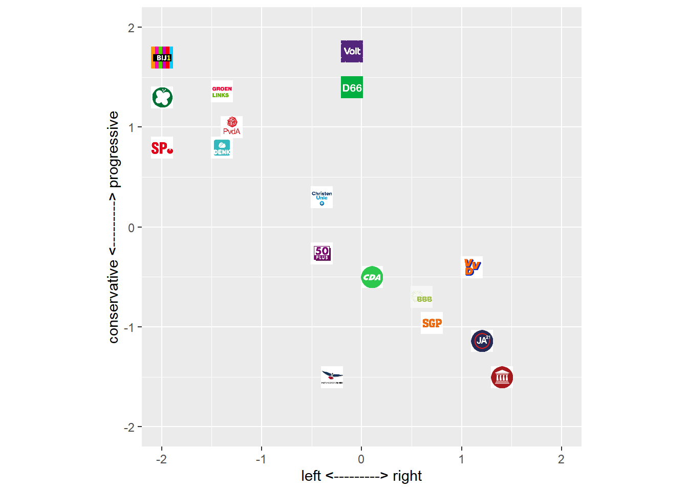

Figure 4.1: Position of Dutch Political Parties in a 2D opinion space

4.3 Baseline polarization

Let us assume that each party would receive a similar vote share, what would be the degree of polarization given the position of these parties in opinion space?

Let us define the vote shares:

votes <- rep(10, 17)

And define the positions:

positions <- (cbind(positions_df$x, positions_df$y) + 2)/4  #range [0,1]
positions

#>        [,1]  [,2]
#>  [1,] 0.000 0.925
#>  [2,] 0.000 0.825
#>  [3,] 0.150 0.840
#>  [4,] 0.000 0.700
#>  [5,] 0.175 0.750
#>  [6,] 0.150 0.700
#>  [7,] 0.475 0.940
#>  [8,] 0.475 0.850
#>  [9,] 0.400 0.575
#> [10,] 0.400 0.435
#> [11,] 0.425 0.125
#> [12,] 0.525 0.375
#> [13,] 0.650 0.325
#> [14,] 0.675 0.260
#> [15,] 0.775 0.400
#> [16,] 0.800 0.215
#> [17,] 0.850 0.125

And calculate the baseline polarization:

fPvar(votes = votes, positions = positions)
fPER(votes = votes, positions = positions)
fPV(votes = votes, positions = positions)

#> [1] 0.3316736
#> [1] 0.02796126
#> [1] 0.5161326

5 Election results

5.1 Input

Let us load the dataset on election results into our environment. This dataset has been constructed and saved here

load("./data/processed/20220625polling_df")
js_df <- x
rm(x)

5.2 Data wrangling

5.2.1 calculating polarization

js_df <- ungroup(js_df)

js_df$Pvar <- rep(NA, nrow(js_df))
js_df$PER <- rep(NA, nrow(js_df))
js_df$PV <- rep(NA, nrow(js_df))

# I will use dimensions as above, but you will need to tweak of course.
positions <- (cbind(positions_df$x, positions_df$y) + 2)/4  #to range 0-1

for (i in 1:nrow(js_df)) {
    votes <- c(js_df$BIJ1[i], js_df$PvdD[i], js_df$GL[i], js_df$SP[i], js_df$PvdA[i], js_df$DENK[i],
        js_df$Volt[i], js_df$D66[i], js_df$CU[i], js_df$PLUS50[i], js_df$PVV[i], js_df$CDA[i], js_df$BBB[i],
        js_df$SGP[i], js_df$VVD[i], js_df$JA21[i], js_df$FvD[i])
    js_df$Pvar[i] <- fPvar(votes = votes, positions = positions)
    js_df$PER[i] <- fPER(votes = votes, positions = positions)
    js_df$PV[i] <- fPV(votes = votes, positions = positions)
}
# you may get a warning, this is because there is no variance at some polling stations

5.2.2 make spatialobject

coords <- js_df[, c("long", "lat")]  # coordinates
crs <- st_crs("+proj=longlat +ellps=WGS84 +datum=WGS84")
js_sp_df <- sf::st_as_sf(x = js_df, coords = c("long", "lat"), crs = crs)

5.2.3 distances between polling stations

We will use these a bit later, when we are going to calculate the spatial correlation of polarization.

# via old package sp
coords <- js_df[, c("long", "lat")]  # coordinates
crs <- sp::CRS("+proj=longlat +ellps=WGS84 +datum=WGS84")
js_sp_df_sp <- sp::SpatialPointsDataFrame(coords = coords, data = js_df, proj4string = crs)
pol_distmat_sp <- sp::spDists(js_sp_df_sp, longlat = TRUE)  #distance in km, ellipsoidal distances?
# pol_distmat_sp[1:10,1:10]

# via new package sf sf_use_s2(FALSE) if you want ellipsoidal distances
pol_distmat <- sf::st_distance(js_sp_df)  #distance in meters, great circle!
# pol_distmat[1:10,1:10]

6 Results

6.1 Correlation of polarization measures

Have a look at the correlations between the different polarization measures.

js_df %>%
    dplyr::select(Pvar, PER, PV) %>%
    as.data.frame() %>%
    cor(use = "pairwise.complete.obs")

#>           Pvar       PER        PV
#> Pvar 1.0000000 0.4076473 0.7730680
#> PER  0.4076473 1.0000000 0.2825026
#> PV   0.7730680 0.2825026 1.0000000

6.2 some polarized polling stations

votes <- cbind(js_df$BIJ1, js_df$PvdD, js_df$GL, js_df$SP, js_df$PvdA, js_df$DENK, js_df$Volt, js_df$D66,
    js_df$CU, js_df$PLUS50, js_df$PVV, js_df$CDA, js_df$BBB, js_df$SGP, js_df$VVD, js_df$JA21, js_df$FvD)
shares <- votes/rowSums(votes)

plotexample <- which(js_df$PER == sort(js_df$PER, decreasing = TRUE)[100])

per100 <- ggplot(positions_df, aes(x, y)) + geom_image(aes(image = image), size = shares[plotexample,
    ]) + xlim(-2, 2) + ylim(-2, 2) + theme(aspect.ratio = 1)


plotexample <- which(js_df$PER == sort(js_df$PER, decreasing = TRUE)[101])

per101 <- ggplot(positions_df, aes(x, y)) + geom_image(aes(image = image), size = shares[plotexample,
    ]) + xlim(-2, 2) + ylim(-2, 2) + theme(aspect.ratio = 1)

plotexample <- which(js_df$PER == sort(js_df$PER, decreasing = TRUE)[102])

per102 <- ggplot(positions_df, aes(x, y)) + geom_image(aes(image = image), size = shares[plotexample,
    ]) + xlim(-2, 2) + ylim(-2, 2) + theme(aspect.ratio = 1)

plotexample <- which(js_df$Pvar == sort(js_df$Pvar, decreasing = TRUE)[100])

pvar100 <- ggplot(positions_df, aes(x, y)) + geom_image(aes(image = image), size = shares[plotexample,
    ]) + xlim(-2, 2) + ylim(-2, 2) + theme(aspect.ratio = 1)


plotexample <- which(js_df$Pvar == sort(js_df$Pvar, decreasing = TRUE)[101])

pvar101 <- ggplot(positions_df, aes(x, y)) + geom_image(aes(image = image), size = shares[plotexample,
    ]) + xlim(-2, 2) + ylim(-2, 2) + theme(aspect.ratio = 1)

plotexample <- which(js_df$Pvar == sort(js_df$Pvar, decreasing = TRUE)[102])

pvar102 <- ggplot(positions_df, aes(x, y)) + geom_image(aes(image = image), size = shares[plotexample,
    ]) + xlim(-2, 2) + ylim(-2, 2) + theme(aspect.ratio = 1)


plotexample <- which(js_df$PV == sort(js_df$PV, decreasing = TRUE)[100])

pv100 <- ggplot(positions_df, aes(x, y)) + geom_image(aes(image = image), size = shares[plotexample,
    ]) + xlim(-2, 2) + ylim(-2, 2) + theme(aspect.ratio = 1)


plotexample <- which(js_df$PV == sort(js_df$PV, decreasing = TRUE)[101])

pv101 <- ggplot(positions_df, aes(x, y)) + geom_image(aes(image = image), size = shares[plotexample,
    ]) + xlim(-2, 2) + ylim(-2, 2) + theme(aspect.ratio = 1)

plotexample <- which(js_df$PV == sort(js_df$PV, decreasing = TRUE)[102])

pv102 <- ggplot(positions_df, aes(x, y)) + geom_image(aes(image = image), size = shares[plotexample,
    ]) + xlim(-2, 2) + ylim(-2, 2) + theme(aspect.ratio = 1)


require(gridExtra)
grid.arrange(arrangeGrob(per100, left = "fPER"), per101, per102, arrangeGrob(pvar100, left = "fPVar"),
    pvar101, pvar102, arrangeGrob(pv100, left = "fPV"), pv101, pv102, layout_matrix = rbind(c(1, 2, 3),
        c(4, 5, 6), c(7, 8, 9)), left = "polarization measure", top = "polling stations")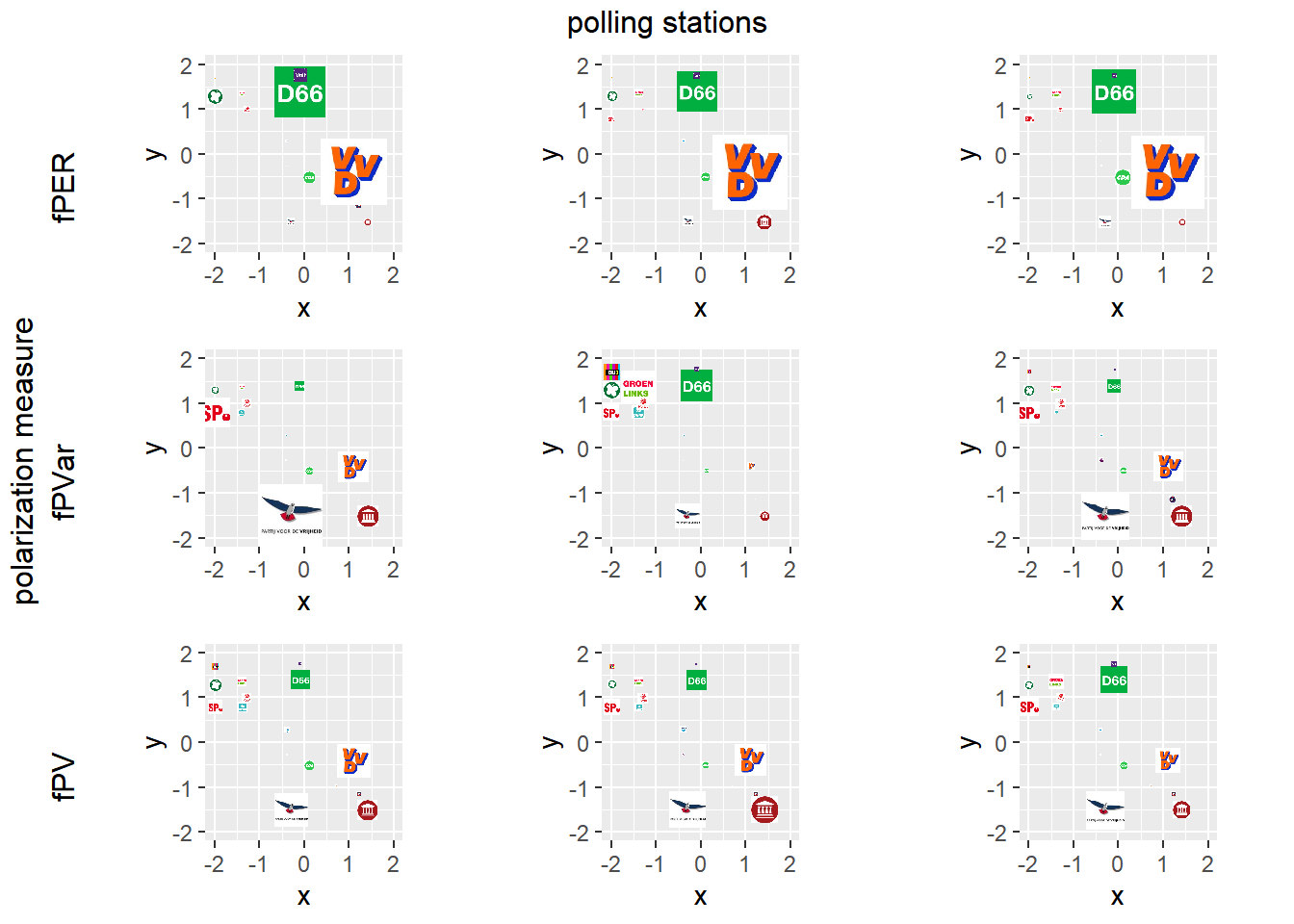

Figure 6.1: Examples of polarized polling stations

6.3 some non-polarized polling stations

votes <- cbind(js_df$BIJ1, js_df$PvdD, js_df$GL, js_df$SP, js_df$PvdA, js_df$DENK, js_df$Volt, js_df$D66,
    js_df$CU, js_df$PLUS50, js_df$PVV, js_df$CDA, js_df$BBB, js_df$SGP, js_df$VVD, js_df$JA21, js_df$FvD)
shares <- votes/rowSums(votes)

plotexample <- which(js_df$PER == sort(js_df$PER, decreasing = FALSE)[100])

per100 <- ggplot(positions_df, aes(x, y)) + geom_image(aes(image = image), size = shares[plotexample,
    ]) + xlim(-2, 2) + ylim(-2, 2) + theme(aspect.ratio = 1)


plotexample <- which(js_df$PER == sort(js_df$PER, decreasing = FALSE)[101])

per101 <- ggplot(positions_df, aes(x, y)) + geom_image(aes(image = image), size = shares[plotexample,
    ]) + xlim(-2, 2) + ylim(-2, 2) + theme(aspect.ratio = 1)

plotexample <- which(js_df$PER == sort(js_df$PER, decreasing = FALSE)[102])

per102 <- ggplot(positions_df, aes(x, y)) + geom_image(aes(image = image), size = shares[plotexample,
    ]) + xlim(-2, 2) + ylim(-2, 2) + theme(aspect.ratio = 1)

plotexample <- which(js_df$Pvar == sort(js_df$Pvar, decreasing = FALSE)[100])

pvar100 <- ggplot(positions_df, aes(x, y)) + geom_image(aes(image = image), size = shares[plotexample,
    ]) + xlim(-2, 2) + ylim(-2, 2) + theme(aspect.ratio = 1)


plotexample <- which(js_df$Pvar == sort(js_df$Pvar, decreasing = FALSE)[101])

pvar101 <- ggplot(positions_df, aes(x, y)) + geom_image(aes(image = image), size = shares[plotexample,
    ]) + xlim(-2, 2) + ylim(-2, 2) + theme(aspect.ratio = 1)

plotexample <- which(js_df$Pvar == sort(js_df$Pvar, decreasing = FALSE)[102])

pvar102 <- ggplot(positions_df, aes(x, y)) + geom_image(aes(image = image), size = shares[plotexample,
    ]) + xlim(-2, 2) + ylim(-2, 2) + theme(aspect.ratio = 1)


plotexample <- which(js_df$PV == sort(js_df$PV, decreasing = FALSE)[100])

pv100 <- ggplot(positions_df, aes(x, y)) + geom_image(aes(image = image), size = shares[plotexample,
    ]) + xlim(-2, 2) + ylim(-2, 2) + theme(aspect.ratio = 1)


plotexample <- which(js_df$PV == sort(js_df$PV, decreasing = FALSE)[101])

pv101 <- ggplot(positions_df, aes(x, y)) + geom_image(aes(image = image), size = shares[plotexample,
    ]) + xlim(-2, 2) + ylim(-2, 2) + theme(aspect.ratio = 1)

plotexample <- which(js_df$PV == sort(js_df$PV, decreasing = FALSE)[102])

pv102 <- ggplot(positions_df, aes(x, y)) + geom_image(aes(image = image), size = shares[plotexample,
    ]) + xlim(-2, 2) + ylim(-2, 2) + theme(aspect.ratio = 1)


require(gridExtra)
grid.arrange(arrangeGrob(per100, left = "fPER"), per101, per102, arrangeGrob(pvar100, left = "fPVar"),
    pvar101, pvar102, arrangeGrob(pv100, left = "fPV"), pv101, pv102, layout_matrix = rbind(c(1, 2, 3),
        c(4, 5, 6), c(7, 8, 9)), left = "polarization measure", top = "polling stations")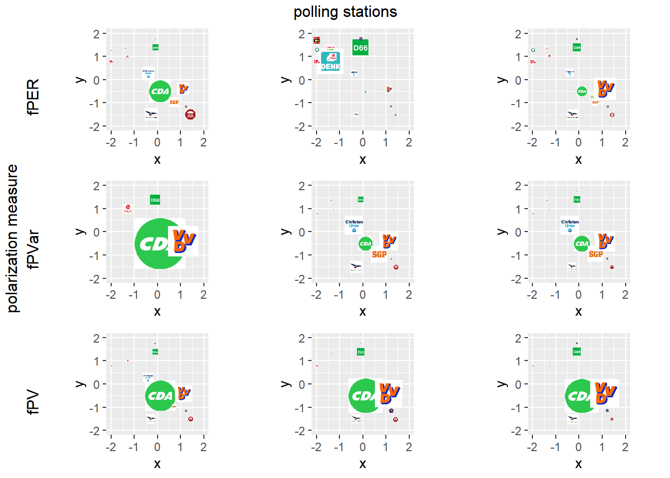

Figure 6.2: Examples of non-polarized polling stations

6.4 Spatial distribution of polarization (graphically)

6.4.1 interactive plot

require("leaflet")

# r.ramp <- rainbow(10) colpol <- cut_number(js_df$PV, n = 10) #make 10 equally sized groups.
# centiles.  js_df$polcol <- r.ramp[colpol] #give these a nice color leaflet(data = js_df) %>%
# addTiles() %>% addCircleMarkers(~long, ~lat, radius=5, color=js_df$polcol)

qpal <- colorQuantile("RdYlBu", js_df$PV, n = 10)
leaflet(data = js_df) %>%
    addTiles() %>%
    addCircleMarkers(~long, ~lat, radius = 5, color = ~qpal(PV)) %>%
    addLegend("bottomright", pal = qpal, values = ~PV, title = "Polarization", opacity = 1)

Figure 6.3: Polarized Polling Stations (leaflet)

6.4.2 static plot

myMap <- ggmap::get_stamenmap(bbox = c(left = min(js_df$long), bottom = min(js_df$lat), right = max(js_df$long),
    top = max(js_df$lat)), crop = FALSE, zoom = 10)

groupPlot <- ggmap(myMap, darken = c(0.5, "white")) + geom_point(aes(x = long, y = lat, color = PV),
    data = js_df, size = 1) + scale_color_viridis_c(option = "A")

groupPlot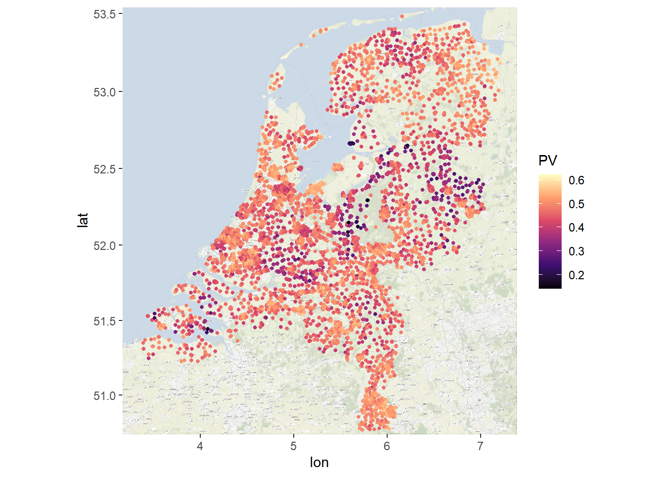

Figure 6.4: Polarized Polling Stations (ggmap)

6.5 Spatial distribution of polarization (formally)

Let us explore whether polling stations with similar levels of polarization are close to each other. Thus phrased otherwise, is there a correlation between the degree of polorization of a polling station i and the degree of polarization of the polling stations in the vicinity of this polling station. We will calculate the spatial correlation measure Moran’s I.

We will discuss Moran’s I here.

We know it is important to make a couple of decisions before hand:

shape of the distance decay function
yes/no row standardization of the weight matrix

6.5.1 distance decay function

We will use an exponential decay function. We will measure distance in kilometer

x <- seq(0.1, 5, 0.1)  #distance
y1 <- exp(-x * 0.5)
y2 <- exp(-x)
y3 <- exp(-x * 2)
y4 <- exp(-x * 3)
x <- rep(x, 4)
y <- c(y1, y2, y3, y4)
s <- as.factor(rep(c(0.5, 1, 2, 3), each = length(y1)))
df <- data.frame(x = x, y = y, s = s)

ggplot(df, aes(x = x, y = y, group = s, col = s)) + geom_line(lwd = 1.2) + labs(title = " ", subtitle = expression(e^{
    -x %*% s
}), x = "Distance (km)", y = "Proximity") + scale_color_discrete(name = "slope (s)")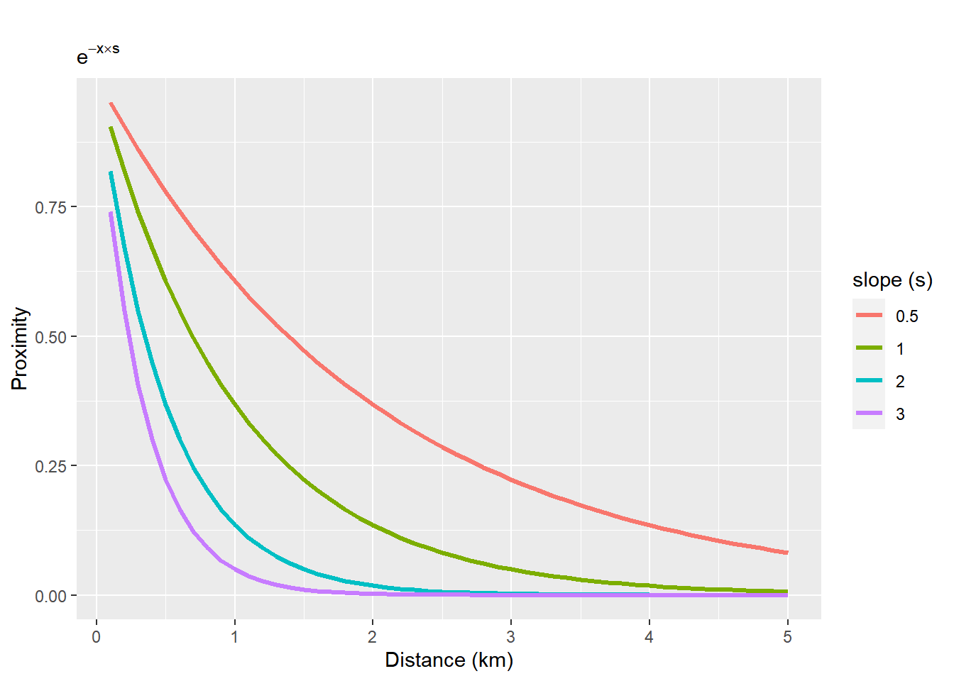

Figure 6.5: Exponential distance decay functions with different slopes

6.5.2 Moran’s I (slope 1)

We already calculated the distances between all polling station, see pol_distmat. Depending on the package this is measured in meters or kilometers, thus be aware!!. Please set to kilometers.

Let us set s to 1.

How to interpret this?

s <- 1
exp(-1 * s)/exp(-10 * s)

#> [1] 8103.084

1km matters 8103 times more than 10km

# I can't get poldistmat to work, reverting to pol_distmat_sp poldistmat <- pol_distmat / 1000 #to
# kilometers poldistmat <- as.matrix(poldistmat) #change object type weights <- exp(-poldistmat)

s <- 1
weights <- exp(-pol_distmat_sp * s)

# we set weight to yourself as zero!
diag(weights) <- 0

print("slope 1, rowstandarize=TRUE")
Ms1 <- fMoranI(x = js_df$PV, scaled = FALSE, weight = weights, na.rm = TRUE, rowstandardize = TRUE)
Ms1$observed

print("slope 1, rowstandarize=FALSE")
Ms1b <- fMoranI(js_df$PV, scaled = TRUE, weight = weights, na.rm = TRUE, rowstandardize = FALSE)
Ms1b$observed

#> [1] "slope 1, rowstandarize=TRUE"
#> [1] 0.628917
#> [1] "slope 1, rowstandarize=FALSE"
#> [1] 0.3457963

6.5.3 Assignment

Whether or not to rowstandardize seems to matter a lot. Do you have any ideas why? Thus, give an interpretation of row standardization. Which measure would you prefer?

6.5.4 Moran’s I (slope 0.5)

Let us make a less steep distance decay function, with s=0.5.

s <- 0.5
exp(-1 * s)/exp(-10 * s)

#> [1] 90.01713

1km matters 90 times more than 10km

s <- 0.5
weights <- exp(-pol_distmat_sp * s)
# for Moran.I we set weight to yourself as zero!
diag(weights) <- 0

print("slope .5, rowstandarize=TRUE")
Ms0.5 <- fMoranI(js_df$PV, scaled = TRUE, weight = weights, na.rm = TRUE, rowstandardize = TRUE)
Ms0.5$observed

print("slope .5, rowstandarize=FALSE")
Ms0.5b <- fMoranI(js_df$PV, scaled = TRUE, weight = weights, na.rm = TRUE, rowstandardize = FALSE)
Ms0.5b$observed

#> [1] "slope .5, rowstandarize=TRUE"
#> [1] 0.5210133
#> [1] "slope .5, rowstandarize=FALSE"
#> [1] 0.2646761

6.5.5 Assignment

A. It seems, that if we also take into account polling stations further away, the correlation becomes weaker. What does this mean?

B. Suppose we would have 100 times as many polling stations, would the difference between the Moran’s I with slope 1 and 0.5 become smaller or larger?

6.5.6 density weighted Moran’s I (slope 1)

It seems a bit strange that we treat small and large polling stations a like. Let us try to correct for that with our modified function of Moran’s I.

s <- 1
weights <- exp(-pol_distmat_sp * s)
diag(weights) <- 0

print("slope 1, rowstandarize=TRUE, not-density corrected")
Ms1 <- fMoranI(x = js_df$PV, scaled = FALSE, weight = weights, na.rm = TRUE, rowstandardize = TRUE)
Ms1$observed

print("slope 1, rowstandarize=TRUE, density corrected")
Mdenss1 <- fMoranIdens(js_df$PV, weight = weights, dens = js_df$Geldige.stemmen/sum(js_df$Geldige.stemmen))
Mdenss1$globalI

s <- 0.5
weights <- exp(-pol_distmat_sp * s)
diag(weights) <- 0

print("slope .5, rowstandarize=TRUE, not-density corrected")
Ms.5 <- fMoranI(x = js_df$PV, scaled = FALSE, weight = weights, na.rm = TRUE, rowstandardize = TRUE)
Ms.5$observed

print("slope .5, rowstandarize=TRUE, density corrected")
Mdenss.5 <- fMoranIdens(js_df$PV, weight = weights, dens = js_df$Geldige.stemmen/sum(js_df$Geldige.stemmen))
Mdenss.5$globalI

#> [1] "slope 1, rowstandarize=TRUE, not-density corrected"
#> [1] 0.628917
#> [1] "slope 1, rowstandarize=TRUE, density corrected"
#> [1] 0.6630065
#> [1] "slope .5, rowstandarize=TRUE, not-density corrected"
#> [1] 0.5210133
#> [1] "slope .5, rowstandarize=TRUE, density corrected"
#> [1] 0.551323

7 Assignment

Optional!! Adapt density Moran’s I so we can turn on/off rowstandardisation.

8 Assignment

Each one of you will have to explain patterns of spatial correlation in one specific city.
A. Explore Spatial correlations in the following ‘parameter space’:
- type of polarization measure
- political position
- type of spatial correlation (for now only Moran’s I, but later perhaps also others)
- yes/no row-standardization
- yes/no density corrected
- different slopes

B. Make plots of the polarization measure for which you disovered the most pronounced spatial correlation(s). See Figures above.

C. Take a close look at your (interactive) plots. Can you derive hypothesis on why polarization did and did/not occur in specific parts

Political Polarization - Polarized Polling Stations